library(tidyverse)
data(starwars)Practical 1
This practical focuses on building scatterplots with ggplot2, then splitting plots into subplots with facets.
All datasets used here are built into R packages.
Create a scatterplot
- Load the
tidyversepackage and thestarwarsdataset.
- Create a scatterplot of
mass(x-axis) againstheight(y-axis).
NoteSolution
starwars |>
  ggplot() +
  aes(x = mass, y = height) +
  geom_point()
Warning: Removed 28 rows containing missing values or values outside the scale range
(`geom_point()`).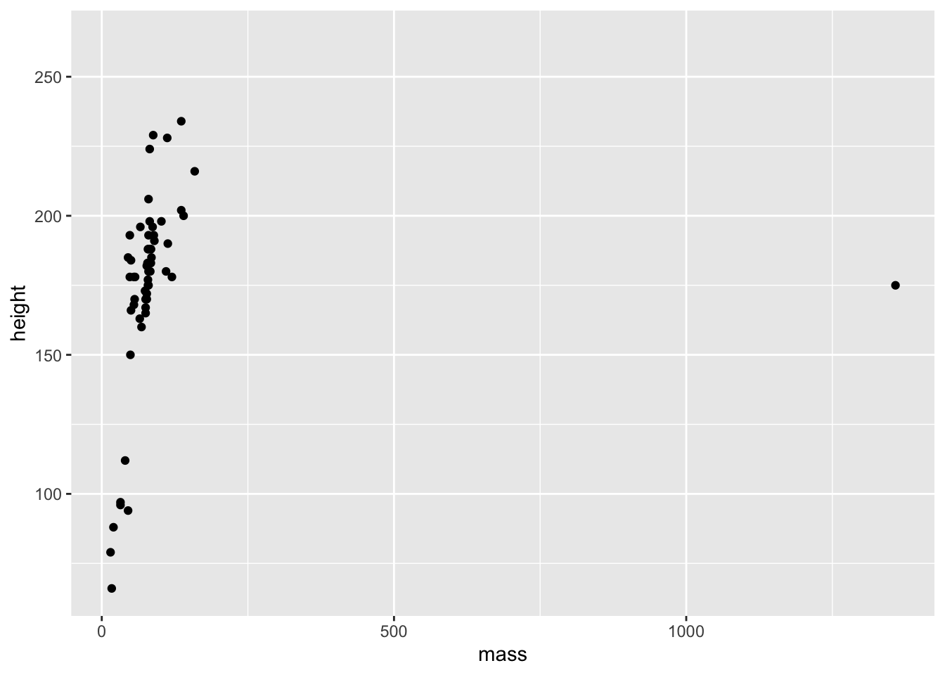
- Remove the outlying point and redraw the plot.
NoteSolution
starwars |>
  filter(mass < 1000) |>
  ggplot() +
  aes(x = mass, y = height) +
  geom_point()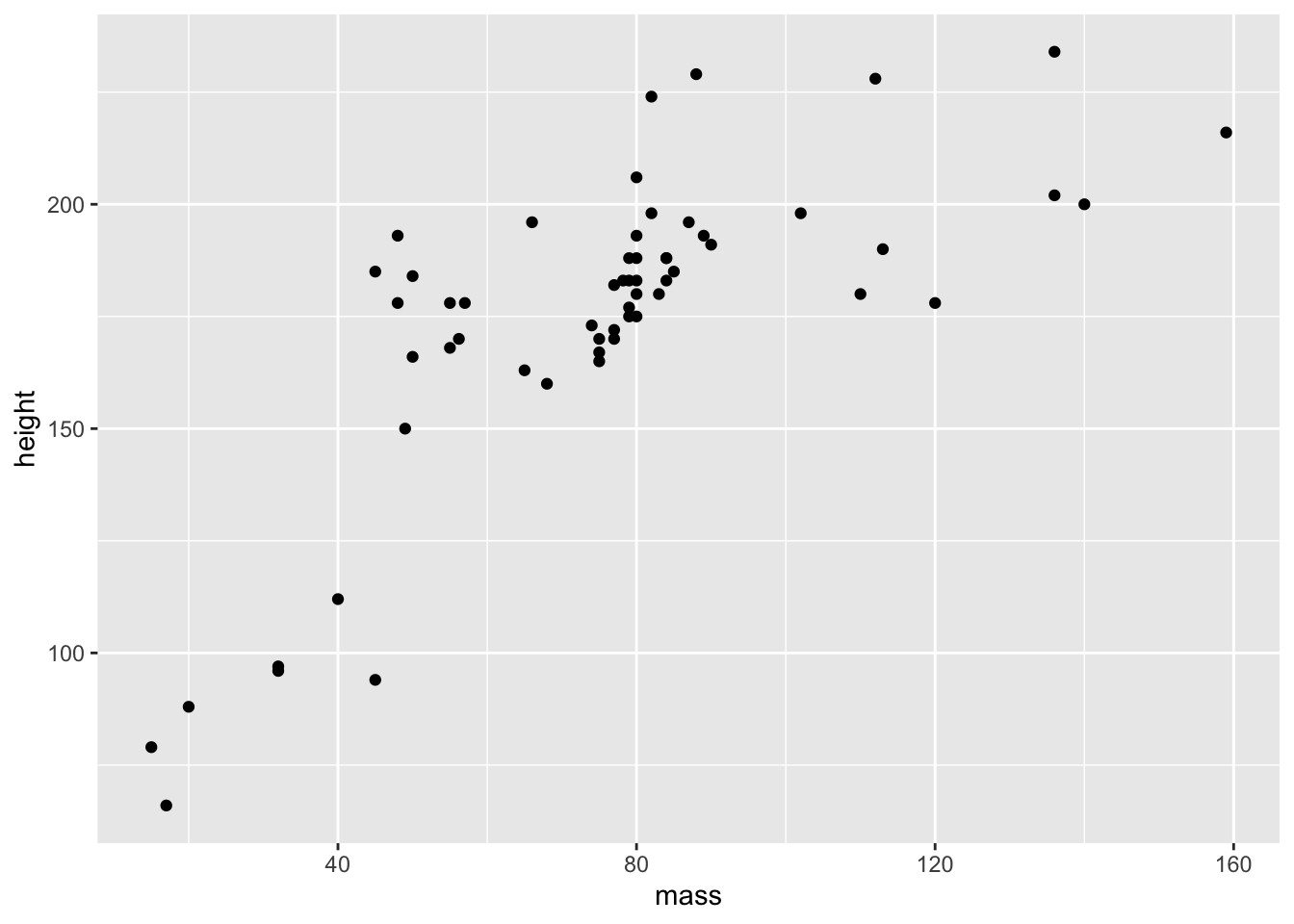
- Color the points by
homeworld.
NoteSolution
starwars |>
  filter(mass < 1000) |>
  ggplot() +
  aes(x = mass, y = height) +
  geom_point(aes(color = homeworld))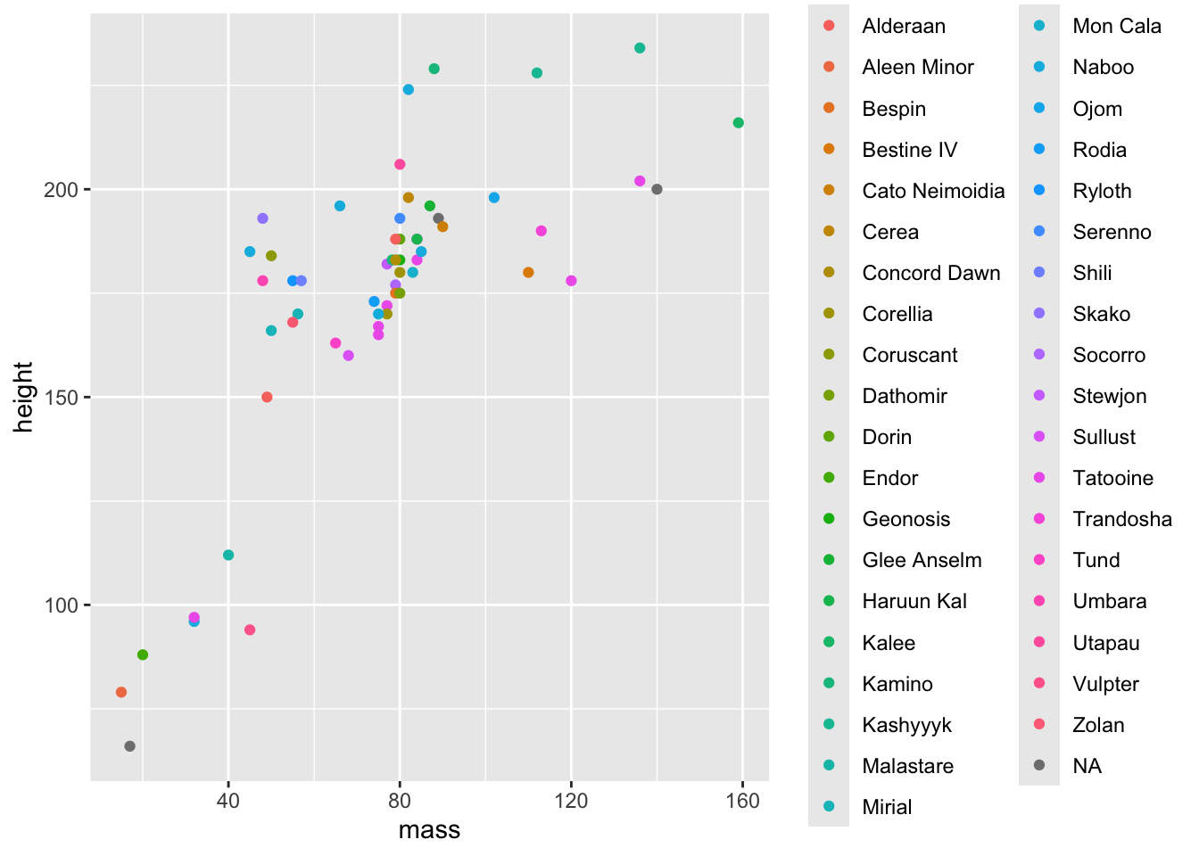
- Add a line-of-best-fit.
NoteSolution
starwars |>
  filter(mass < 1000) |>
  ggplot() +
  aes(x = mass, y = height) +
  geom_point(aes(color = homeworld)) +
  geom_smooth(method = "lm") +
  theme(legend.position = "none")
`geom_smooth()` using formula = 'y ~ x'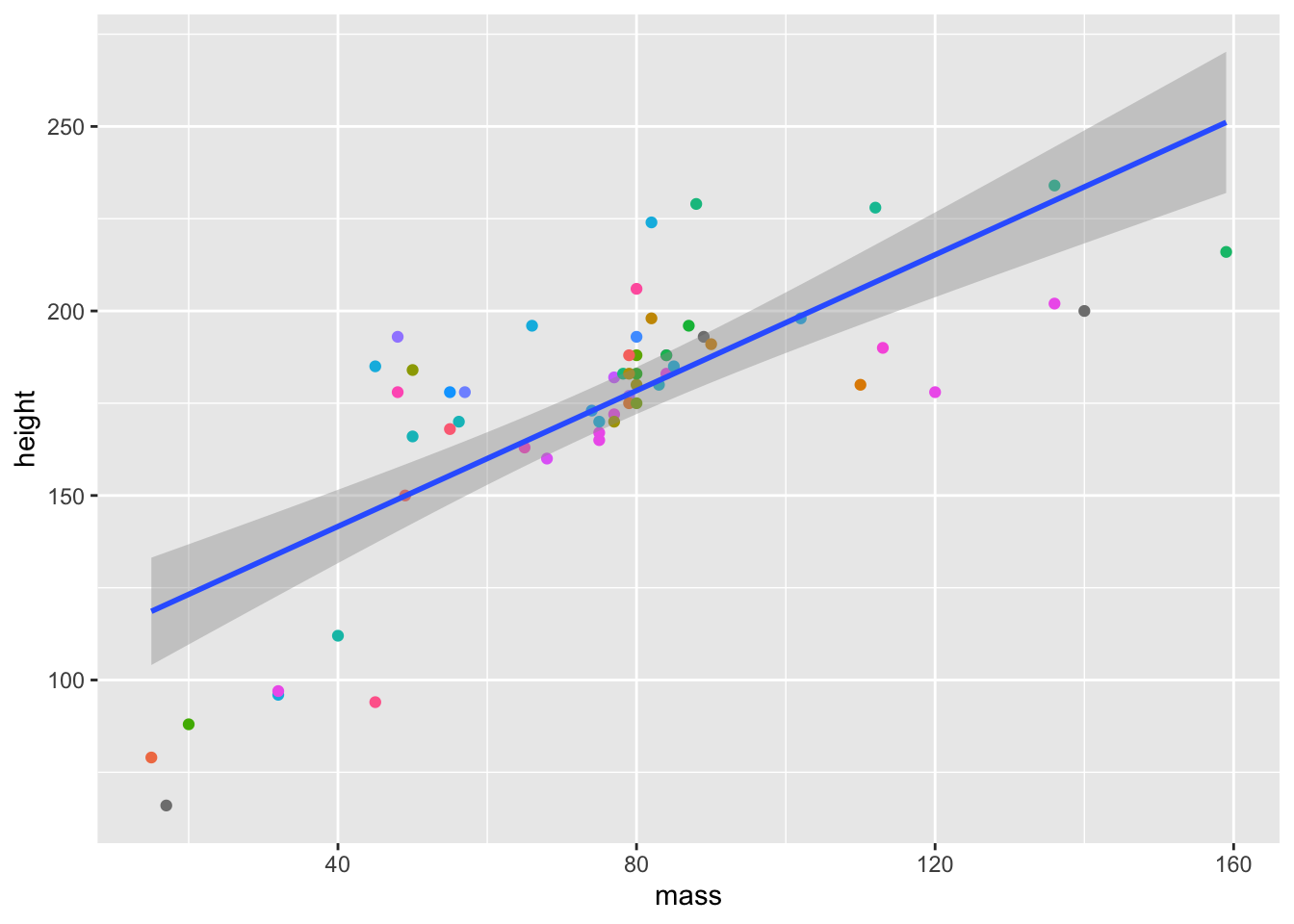
Facets with facet_wrap
- Load the
mtcarsdataset.
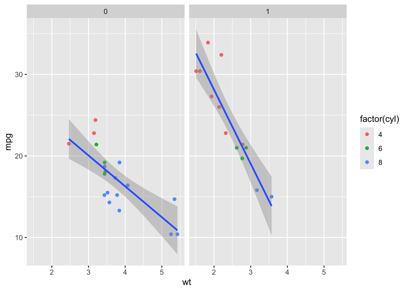
data(mtcars)- Create a scatterplot of
wtagainstmpg. - Color the points by
cyl. - Add a line-of-best-fit.
- Produce separate plots for automatic and manual cars (
am).
NoteSolution
mtcars |>
  ggplot() +
  aes(x = wt, y = mpg) +
  geom_point(aes(color = factor(cyl))) +
  geom_smooth(method = "lm") +
  facet_wrap(~ am)
`geom_smooth()` using formula = 'y ~ x'